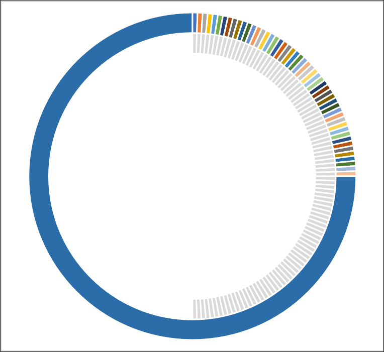
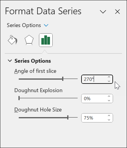
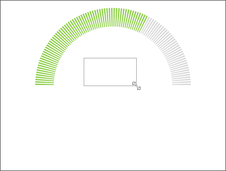
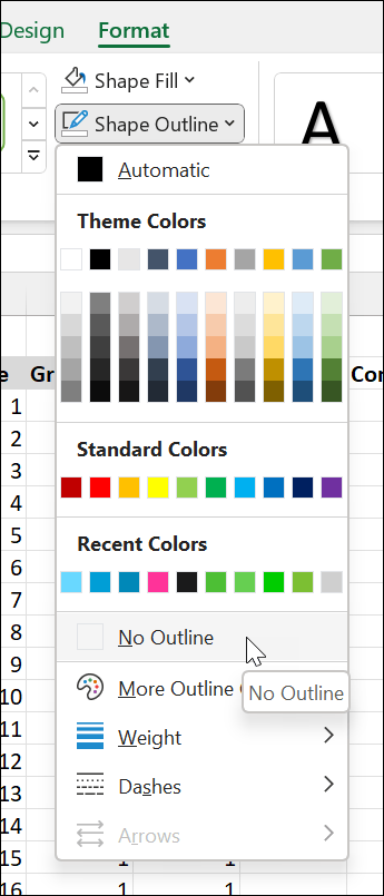
This video has been updated to incorporate a better and easier way to build out this chart, thanks to a suggestion from my friend Jon Peltier from peltiertech.com. If you watched the original video that was released on September 6, be sure to watch again for updated content.
I asked readers to tell me which chart was their favorite. To my surprise, one of the leading charts in popularity was the Gauge Chart.
The gauge chart shows percent completion to 100% on a half circle. Or in the case of a gas gauge, it can show consumption until empty. This chart that we're going to create is actually half of a Donut Chart
Why did this particular chart get so many votes? A gauge chart is something we've all seen on the dashboard of a car or a pressure valve, so it's familiar to our brains and easy to read. Also, the circular shape draws our eye, especially amid squares, lines, and rectangles.
Boring Gauge Chart
Before we begin building this chart, you should know that you can easily create one that doesn't have the incremental lines. I call it the Boring Gauge Chart, but if you like the look better, you are welcome to use it.
Creating a Gauge Chart
My preference is to have incremental lines in my gauge chart, where each increment represents one percent of the total.
Let me walk you through how to make this chart, step by step.
Getting Started
Highlight the data for both the Grey and Colored columns (L2:M103). Now go to the Insert tab. Under the Pie Chart dropdown, select the Doughnut chart.
This will create a chart that needs some formatting. Remove the Legend and the Chart Title so only the donut is visible. Resize as needed.
Data Set-Up
Before continuing, let me explain the data set-up. I've created three columns: Sequence, Grey, and Color. The Sequence contains every number from 1 to 100. For the Grey column, every entry has a 1. These represent the 100 increments of our gauge. This is followed by a cell containing the number 100, which represents the half of the donut we don't want to see. We will make that half invisible as we build the chart
For the Color column, I've created a formula using the IF function that changes the value from 1 to 0 depending on the value indicated in a box labeled “Complete.” If the value of the increment is below or equal to the completed amount, it returns a 1, and if it is above, it returns a 0. (You can learn more about writing IF functions here: IF Formula Tutorial for Excel.)
Like the grey circle, this colored circle is completed by the last cell in the data column, which subtracts the “Complete” amount from 200.
If you are confused about why we have a total of 200 when we're only interested in increments from 1 to 100, it's because we are modifying a donut chart (which is a full circle) to look like a gauge chart (which is a half circle), so the second 100 of our 200 is essentially filler. We will make that filler invisible when we format the chart.
Formatting the Chart
Click within the inner donut to select the “Grey” series. Then, go to the Format tab, and choose a grey color in the Shape Fill dropdown. Your donut will now look like this:
Now you want to select the left half of that grey ring. This is the section that's called “Series ‘Grey' Point 101” in the Chart Elements field on the Ribbon.
Once that portion is selected, choose No Fill from the Shape Fill menu. Your donut looks like this now:
Repeat these steps with the outer ring, choosing a color of your preference instead of grey. I chose green. Your donut should look something like this:
Overlapping the Two Series
The next step is to combine our two donuts, overlapping the two series.
With the chart selected, go to the Chart Design tab and choose Change Chart Type. That will open up a window that shows our current selection as a Pie Chart. Select Combo instead.
Then change the chart type for both Grey and Color to Doughnut. Uncheck the Secondary Axis box for Grey and check it for Color.
After you hit OK, your donut will look like this.
Rotate the Chart
The next step is to rotate our donut 270 degrees so that the striped portion is on top. You can rotate it by selecting the Grey series, clicking Format Selection on the Format tab, and changing the Angle of First Slice to 270 on the pane that appears. Repeat this process for the Color series.
Your donut will now look like a gauge chart.
Changing the Thickness
If you want to make the gauge thicker or thinner, you certainly can do that as well. You simply have to decrease or increase the size of the donut hole for both charts. That option is found on the same pane where we rotated the chart.
Adding the Percentage Label
To add a label that shows the number percentage that corresponds to the colored gauge, we will create a text box. Go to the Insert tab, choose Shapes, and select the Text Box shape. That will change your cursor so that you can drag open a text box wherever you choose.
With the border of your new text box selected, go to the formula bar and type =, then select the box that has the percentage complete. That will link your textbox to the cell so that it automatically changes when the percentage changes. Be sure to center, format, enlarge, color, and/or align the text to your liking.
Watch the video tutorial above to see the format changes step by step.
Removing the Border
I like to remove the border from these charts so that it doesn't draw attention to the fact that the lower half of the chart is blank. By removing the border, it appears that there is no lower half and that the entire gauge chart consists of the semi-circle at the top.
To remove the border, simply select the chart, then go to the Format tab. Choose No Outline on the Shape Outline menu.
Conclusion
I hope that this tutorial has been helpful for you. I will be creating tutorials for the other seven progress charts shown above, so stay tuned for those. Feel free to leave any questions or feedback in the comments below!
Excel Campus LLC, 412 Olive Avenue, Suite 315, Huntington Beach, CA 92648, United States
You are receiving this email because you are a valued member of the Excel Campus community. The goal of these emails is to help you learn Excel so you can save time with your everyday tasks and advance in your career. You can unsubscribe at any time by clicking the link below.